Digital images, integral and differential operators are usually stored in matrix form. These matrices are often very large systems and require enormous memory and processing power. In numerical linear algebra, mathematicians are interested in developing algorithms that can efficiently reduce storage without losing too much accuracy. This field is known as low rank approximation.
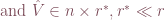
Many matrices that arise from partial differential equations or integral equations are low rank systems because of translational invariance. The most famous and probably most well known low rank approximation algorithm is the singular value decomposition method. Given a matrix  , we can decompose A into the product of three matrices in the form of
 ,
,
where  ,
,  , and
, and  . In this setting,
  is a diagonal matrix and its entries are called the singular values. By convention, the singular values are listed in decreasing order along the diagonal of S. In many systems, the relative magnitude of singular values decays very quickly:

for large  . For this reason, we can approximate the matrix
  by only using the first few singular values. We can write
 ,
,
where  ,
, ,
, . One can prove that singular value decomposition yields the best possible low rank approximation in the Frobenius norm, however this method is computational costly and sometimes numerically unstable. Instead, we introduce a much more efficient method: skeleton decomposition.
The idea is fairly simple, we can rewrite as
 ,
,
where  is the column restriction of
  ,
,  is the row restriction of , and
  is the intersection of row and column restriction. In another word, if has rank
  , then we pick
  columns from and form a submatrix, and then we pick rows from and form a submatrix. Finally, the intersection of and gives
  . The figure below illustrates this process.
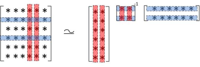
Skeleton decomposition: ,
This method does not need much computation, since we are simply picking rows and columns! The question is how do we pick the best rows and the best columns? This is actually a quiet interesting optimization problem. It turns out that we want to pick the rows and columns that maximize the spanned volume. In another words, we maximize  . Now this question looks like the maximum ellipsoid problem we have on problem set 3. There are multiple iterative algorithms that search for the optimal set of rows and columns. Look into adaptive/ incomplete cross approximation methods for details.
Reference
http://math.mit.edu/icg/papers/sublinear-skeleton.pdf
Written by Yufeng (Kevin) Chen

