Jordan Smith and Soren Larson
Abstract
Modeling in atmospheric transport, astrophysics, diagnostics, genomics, materials science, engineering, and a variety of other systems face a significant constraint in optimizing the distribution of computing power and process sequences in order to appropriately represent forward and inverse model states. Once data is obtained, a vast amount of computational power is necessary to study these relationships. Improved methods of appropriately discerning optimal substructures have the potential to significantly reduce required computational resources while preserving a high degree of overall model accuracy.
Dimension reduction has been well-received as a means of producing cost-effective representations of large-scale systems. In order to reduce the total number of calculations necessary to model a time series in high-dimensional space, methods of extrapolation are commonly used by practitioners as a means by which to reduce computational expense. In these instances, the discretization of partial differential equations (PDEs) aids in optimal control, probability analysis, and inverse problems requiring multiple iterations of system simulation. This iterative approach necessitates that the reduced model produce an accurate representation of the system across a large number of parameters. Dynamic programming has contributed to these model acceleration methods through the isolation of identical problems normally solved many times by the model, known as overlapping sub-problems.
An illustration of the advantages afforded by the implementation of select methods described is simulated using an atmospheric chemical transport application. A global atmospheric model is constructed using empirical time-series data from the Emissions Database for Global Atmospheric Research (EDGAR), and the concentration of chemical species is determined using inverse modeling. In order to improve computation performance, the Jacobian matrix is optimized using a quasi-Newton variable metric algorithm. The model then produces a representation of chemical species concentration in different hemispheres and atmospheric layers across time at significantly reduced computational cost.


Use of a Jacobian matrix and spatial reduction both compartmentalize a given model into two separate regions, with independent variables being solved at each time step and dependent variables either relying upon a system of PDEs or being identified as overlapping sub-problems and subsequently eliminated entirely by dynamic programming. As one or more regions of the system run the model at a normal speed (“fast”) using conventional modeling methods and solving the full mechanism of all equations , other sections run pre-specified components of the model at an accelerated speed using extrapolation (“slow”). These functions both lead to PDEs, requiring numerical analysis techniques to arrive at an optimal solution. The separate sections are then paired in order to extrapolate basic knowledge of the system without having to run every component of the model, substantially reducing computational strain and overall run-time.
The most pronounced drawback of spatial reduction models is that the nature of extrapolation produces additional error, and can lead to highly inaccurate results over the course of the model due to compounding. When applied to models involving time series in high dimensional space, the error produced by extrapolation is often too high to justify the computational savings. For this reason, successful implementation of spatial reduction models has been limited to those with an advanced understanding of the underlying system, in this case primarily geophysicists with atmospheric transport modeling expertise. Improvements in constraining this error without excessive manual adjustments to the model can be achieved by isolating optimal substructures and introducing a trainer.
Application
A large-scale system with some dynamical substructures is desirable for the purposes of examining the range and degree of impact of the algorithm framework relative to both basic extrapolation and standard computation methods. Though generally applicable to many natural sciences systems, this analysis shall focus upon a global atmospheric modeling application due to the expansive size and diverse nature of the system, constant geophysical laws, variety of chemical species, recognizable regions, presence of overlapping substructures, and ease of discretization.
This simulation considers the long-lived greenhouse gas 


Atmospheric concentration of 
Linear transport coefficients were optimized by in-situ concentration observations of 
The Jacobian is ideal in dynamical systems for which and for inverse functions, and can be plainly written as ![(J_{F^-1})(F(p)) = [(J_F)(p)]^{-1}](https://s0.wp.com/latex.php?latex=%28J_%7BF%5E-1%7D%29%28F%28p%29%29+%3D+%5B%28J_F%29%28p%29%5D%5E%7B-1%7D&bg=ffffff&fg=774553&s=0&c=20201002)


The Jacobian relates to a first order Taylor expansion 


For these reasons, the Jacobian is used commonly in global physical sciences modeling. In the application used for this project, the first and second order derivatives of independent variables are known. In such scenarios, most mainstream atmospheric models simply use the Jacobian to create a PDE matrix, solve the inverse problem, and adjust parameters as necessary to obtain a highly accurate fit.
After an initial estimate of the parameter values, the Jacobian matrix is constructed, and the standard objective function 

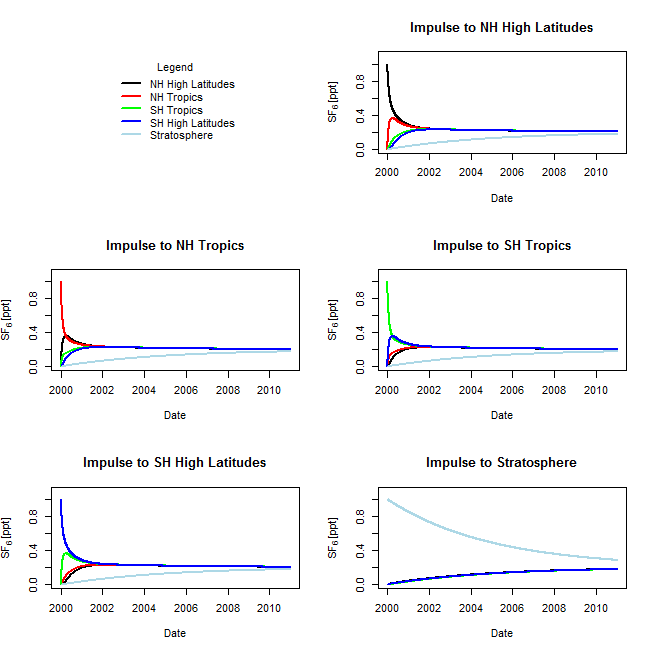
Here the Jacobian itself is performing a reduction function in that the configuration of partial derivatives creates a system in which dependent variables are already being partitioned as overlapping sub-problems and computational resources are not being expended upon optimizing them. A Nelder-Mead algorithm is then implemented in order to find the optimal initial starting chemical species concentration in each of the atmospheric layers.

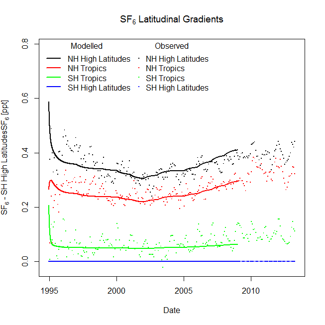
Given the inverse has now been established and the optimal parameters are known, the model is run and compared to empirical data from the Intergovernmental Panel on Climate Change (IPCC). The values are found to be consistent for

Evaluating means of reducing computational expense, a scenario is presented in which no in-depth familiarity with the system is assumed. A trainer and Greedy algorithm are then used in a vector autoregression (VAR) scenario in an attempt to reduce computational expense.
Findings
The inverse model accurately reflects the time-series concentrations of
Recommendations for spatial reduction techniques going forward include increased specification in trainers, ranking/weighting depending upon past performance and known correlations or other period/parameter-specific relationships, use of partial derivatives as a prompt to sample from true observations in areas of decreased stability, and improved means of isolating optimal substructures.
